Theory of Aqueous Solubility Prediction

This documentation provides the theoretical background of Chemaxon's Solubility Predictor.

Table of Contents

• Introduction
• Intrinsic solubility
  • Intrinsic example
• pH-dependent solubility
  • pH-dependent example
• Derivation of the pH-dependent solubility
  • Derivation example
• Cutting off the pH-dependent solubility curve
  • Cut-off examples
• Examples of predicted pH-dependent logS curves
  • Example 1
  • Example 2
  • Example 3
• Test results
• References

Introduction

Aqueous solubility is one of the most important physico-chemical properties in modern drug discovery. It has impact on ADME-related properties like absorption, distribution and oral bioavailability. Solubility can also be a relevant descriptor for property-based computational screening methods in the drug discovery process. Hence there is a significant interest in fast, reliable methods of predicting solubility in water for promising drug candidates.

The two most common types of solubility that can be predicted are intrinsic and pH-dependent solubility.

The most widely accepted and used unit of measuring solubility is logS. It is defined as the 10-based logarithm of the solubility measured in mol/l unit, so logS = log (solubility measured in mol/l).

Intrinsic solubility

The intrinsic solubility of an ionisable compound is the solubility that can be measured after the equilibrium of solvation between the dissolved and the solid state is reached at a pH where the compound is fully neutral. It is usually denoted as logS₀.

Intrinsic example

The intrinsic solubility of phenol can be measured at pH 6.0. Phenol is a weak acid with a pK_a value of 10.02, which means that at pH 6.0 the molecule is dominantly present in its neutral form. So at pH 6.0 equilibrium can be measured only between the solid and the dissolved neutral form.

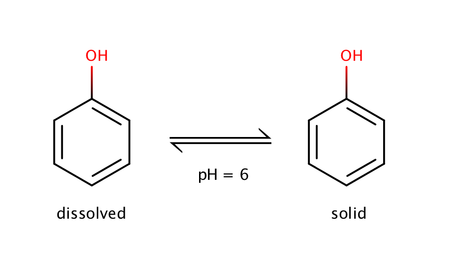
Fig. 1. Solvation equilibrium of phenol at pH 6.0

Our predictor uses a fragment-based method that identifies different structural fragments in the molecule and assigns an intrinsic solubility contribution to them. The contributions then are summed up to determine the intrinsic solubility value. The implementation of the fragment-based method is based on the article of Hou et al.

The figure below shows a molecule split up into fragments that are used to determine the intrinsic solubility.

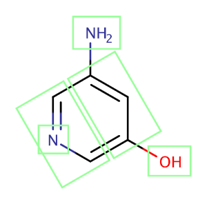
Fig. 2. A molecule split into fragments to determine its intrinsic solubility

pH-dependent solubility

The pH of a solution affects the ionisation of the dissolved compound, shifting its solvation equilibrium. With increasing ionisation solubility increases compared to the intrinsic solubility. Therefore solubility depends on the solution pH. This pH-dependent solubility is usually denoted as logS_pH or simply logS.

pH-dependent example

The solubility of aniline in an acidic environment will be greater than its intrinsic solubility as the protonation of the compound shifts the equilibrium between the pure liquid aniline and its dissolved form to the solvation side (to the dissolved form).

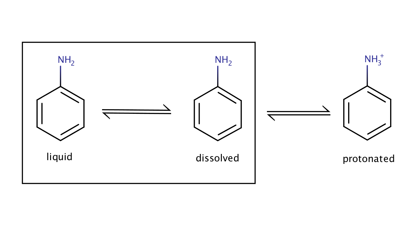
Fig. 3. Solvation equilibrium of aniline in an acidic environment

Derivation of the pH-dependent solubility

The pH-dependent solubility can be derived from the Henderson-Hasselbalch equation and the definition of intrinsic solubility.

In case of a monoprotic acid the formula is the following:

logS_pH = logS₀ + log(1 + 10^(pH-pKa))

For multi-protic compounds the formula can be generalised:

logS_pH = logS₀ + log(1 + α), where α = ∑_iα_cAi/∑_jα_nAj,

where α_cAi is the distribution % of the i-th charged microspecies at the given pH and α_nAj is the distribution % of the j-th neutral microspecies at the given pH.

Derivation example

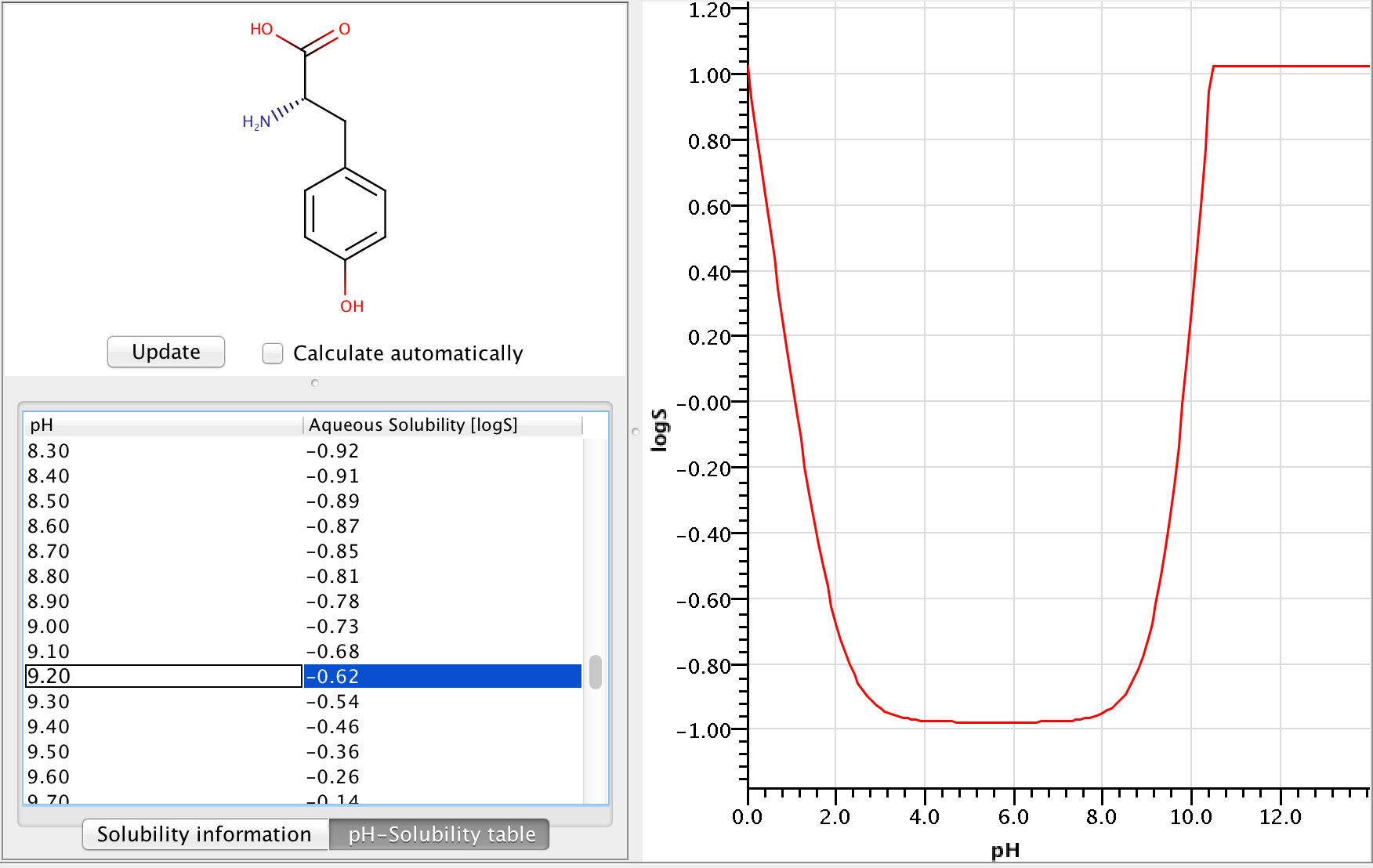
Let's calculate the pH-dependent solubility of L-tyrosine at pH=9.2.

Zwitterionic molecules are the least soluble around their isoelectric point. The predicted isoelectric point of L-tyrosine is 5.5, which means that we can expect higher solubility at pH 9.2 than at pH 5.5.

To get the pH-dependent solubility we first need the intrinsic solubility of L-tyrosine. The logS Predictor predicts -0.98 logS for intrinsic solubility.

To take ionisation into account we have to calculate the microspecies distribution of L-tyrosine at pH=9.2. For that we use the pK_a Plugin, which can also calculate the microspecies distribution based on the predicted pK_a values. The following image shows the output of the plugin, with the highlighted row showing the distributions at pH 9.2.

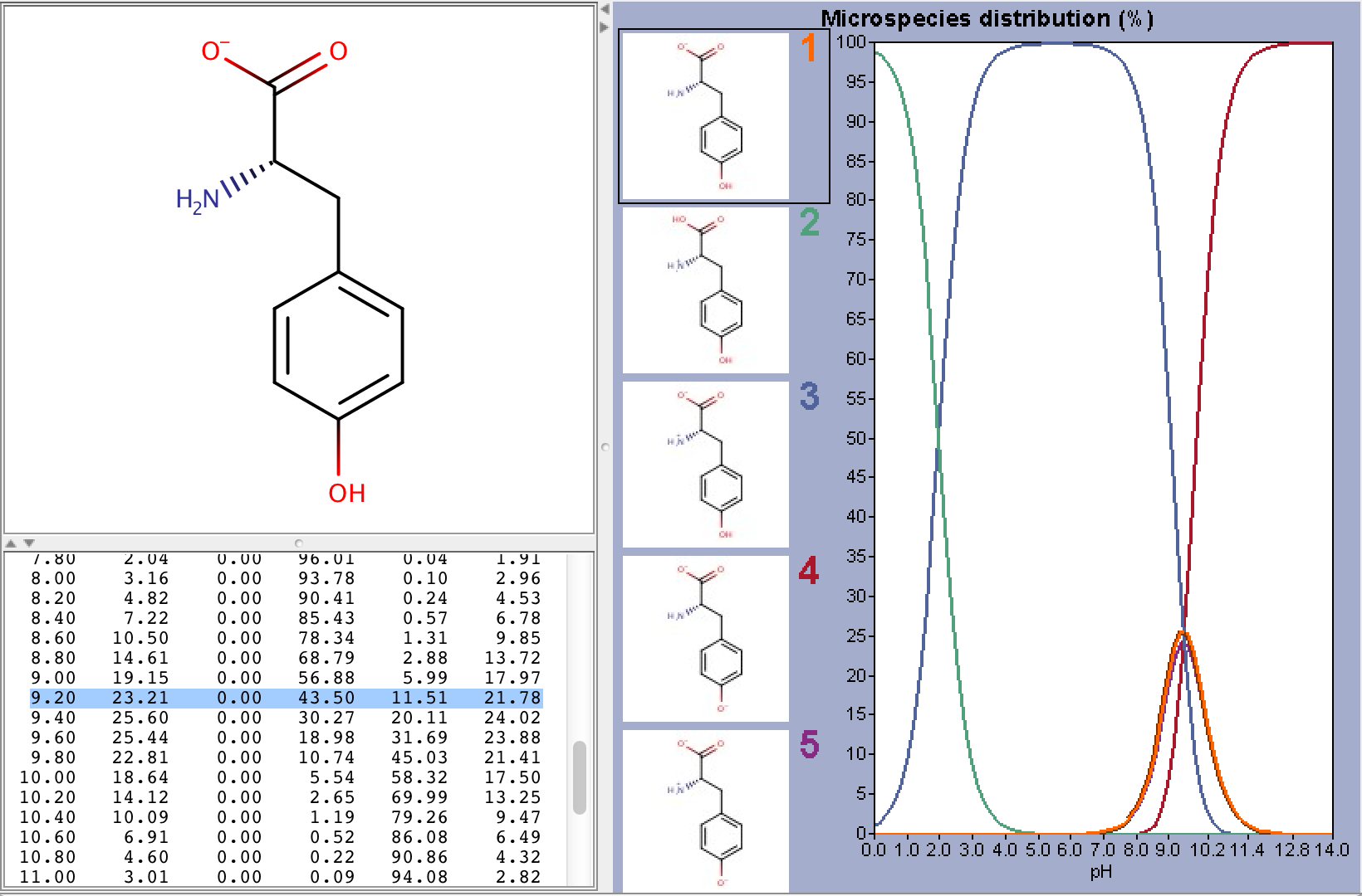
From the image above we can read that the distribution %s of the charged microspecies are (with their charges shown):

23.21 (-1), 0.0 (+1), 11.51 (-1, 1), 21.78 (-1, -1, +1)

The distribution % of the neutral microspecies:

43.50 (zwitterionic species)

Using these we can easily calculate the log(1 + α) correction:

log(1 + α) = log(1 + (23.21 + 0.0 + 11.51 + 21.78)/43.5) = 0.362

Adding the correction to the intrinsic solubility, we get that the pH-dependent solubility at pH 9.2 is -0.618 logS.

The following image shows the full pH-logS curve of tyrosine with the calculated solubility at pH 9.2.

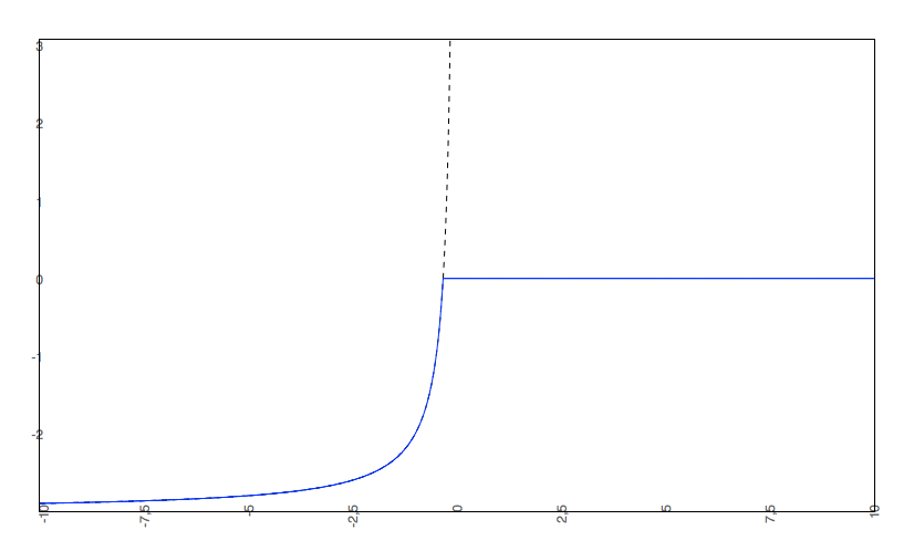
Cutting off the pH-dependent solubility curve

In practice the solubility curve has limits as the solution reaches its saturation. To match the predicted pH-dependent solubility curve to the the real/experimental curve, a cut-off is applied to the predicted curve.

In our logS Predictor we apply the following cut-off (solubility values are expressed in logS unit):

• if the predicted logS₀ > -2, the applied cut-off is +2, which means that the pH-dependent logS curve has a limit value at logS₀ + 2. This means that the pH-dependent logS values cannot increase above logS₀ + 2.

• if the predicted logS₀ < -2, the predicted pH-dependent solubility curve is not be allowed to rise above 0, so the cut-off is at 0.

Cut-off examples

1. The predicted intrinsic solubility (to which value the pH-dependent logS curve converges) is -1.0. Therefore the pH-dependent curve is cut off at +1.0.

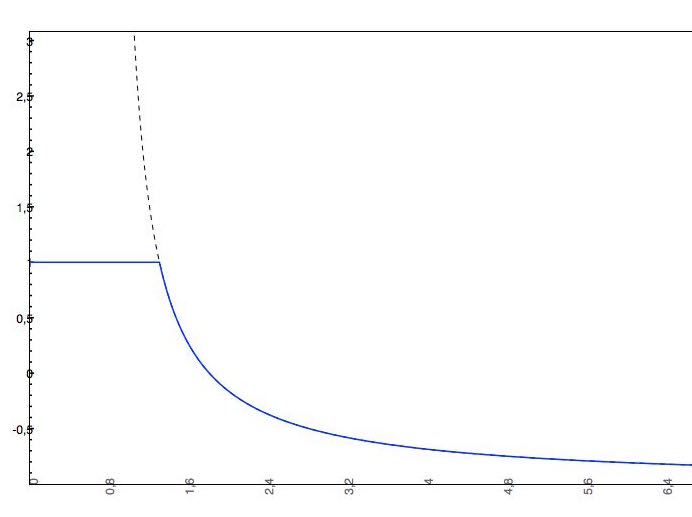
1. The predicted intrinsic solubility (to which the pH-dependent logS curve converges) is -3.0. Therefore the pH-dependent curve is cut off at 0.

Examples of predicted pH-dependent logS curves

In this section you can find some examples of comparing predicted and experimental pH-dependent logS curves for specific drug molecules. The experimental values and the detailed analysis of the experimental logS curves can be found in the referenced literature.

Example 1

The predicted pH-dependent logS curve of the HCl salt of ticlopidine shows a good correlation with the experimental curve, meaning that the HH-equation quite accurately describes the pH-dependence of the solubility. This result also comes from the fact that ticlopidine is a monoprotic base so the HH-equation works well.

The predicted logS₀is -3.47, while the experimental logS₀ is -4.25. The absolute difference between the experimental and predicted intrinsic solubility is 0.78 logS unit.

Example 2

The predicted pH-dependent logS curve of the hydrogen fumarate salt of the diprotic base quetiapine shows good correlation with the experimental curve. Its predicted logS₀ is -4.27, while the experimental logS₀ -2.84. The absolute difference between the experimental and the predicted intrinsic solubility is 1.42.

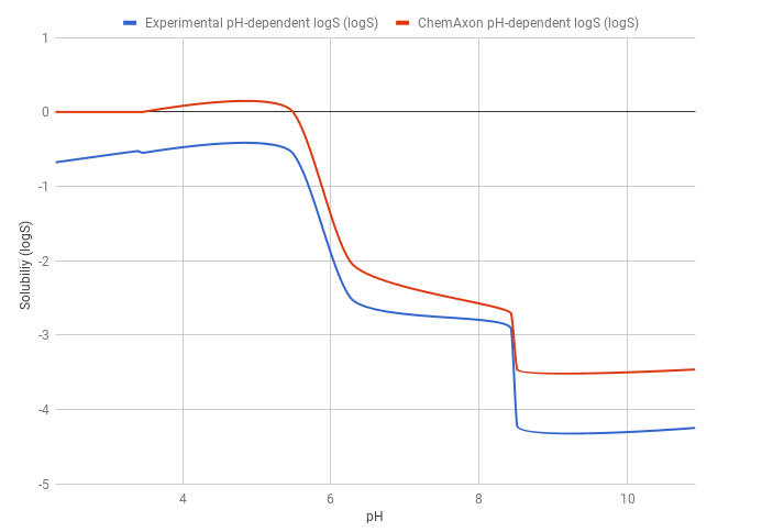
Example 3

The predicted pH-dependent logS curve of the H fumarate salt of the ampholytic desvenlafaxine differs from the experimental curve below pH 6, which is due to salt formation. The predicted intrinsic logS is -2.16, while the experimental is -3.25. The absolute difference between these two values is 1.09 logS unit.

Test results

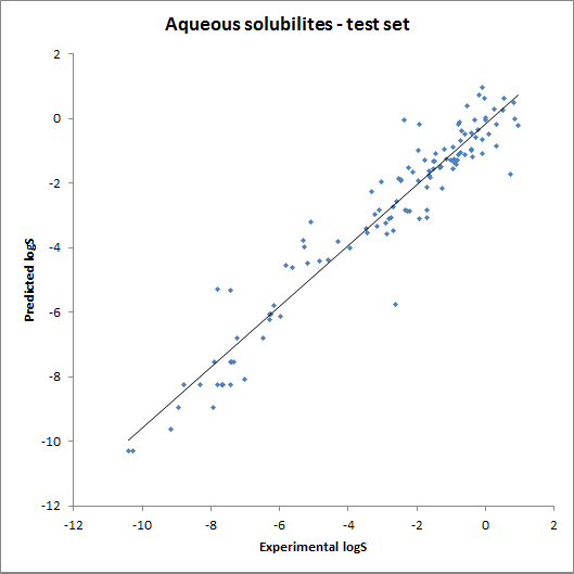
The accuracy of the model was tested using fragment contributions calculated from the training set with a linear regression model. The obtained contributions were then used for calculating solubility for the training and the test set. The results are summarised on the following two charts:

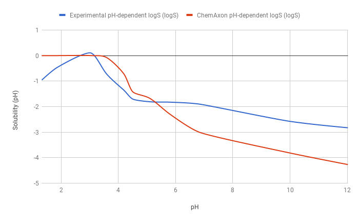
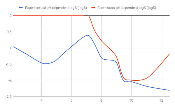
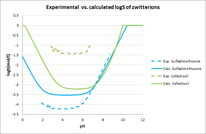
Tests for pH-logS curves were also run. The two plots below show calculated and experimental pH-logS curves for different acidic, basic and zwitter-ionic compounds:

 The Solubility Predictor will be developed further in the future. Among our future goals we have extending the prediction with a descriptor-based method and adding training features.

References

1. Hou, T. J.; Xia, K.; Zhang, W.; Xu, X. J. ADME Evaluation in Drug Discovery. 4. Prediction of Aqueous Solubility Based on Atom Contribuition Approach. J. Chem. Inf. Comput. Sci. 2004, 44, 266-275

2. Völgyi, G.; Baka, E. et al. Study of pH-dependent solubility of organic basis. Revisit of the Henderson-Hasselbalch relationship. Analytica Chimica Acta 2010, 673, 40-46

3. Avdeef, A. et al. Equilibrium solubility measurement of ionizable drugs - consensus recommendations for improving data quality. ADMET & DMPK 4(2) 2016, 117-178

4. Shoghi, E.; Fuguet, E.; Bosch, E.; Rafols, C. Solubility-pH profiles of some acidic, basic and amphoteric drugs. European Journal of Pharmaceutical Sciences 2013, 48, 291-300