API Usage

This manual serves as API Developer and User Guide of JChem PostgreSQL Cartridge (JPC). See also Getting started guide for easy setup and use cases.

If you are familiar with JChem Oracle Cartridge (JOC) and are interested in the differences between JOC and JPC, see their comparison here.

Please be sure, the chemical knowledge behind this API is the same as the knowledge used by JChem Base. In the background of the chemical structure searches, the same molecular comparisons, transformations, calculations are executed as in the case of JChem Base. The differences are collected here.

• CREATE TABLE
  • Prerequisites

• INSERT INTO TABLE

• MOLECULE INDEX

  • How to monitor the CREATE INDEX process

• MOLECULE IMPORT

  • Import from SD file
    ​

    • Import from (cx)smiles or (cx)smarts files
    • Convert molecule source text to molecule from an existing table

• MOLECULE EXPORT

• CACHE LOADING

• MOLECULE FUNCTIONS

  • Casting a string to any Molecule type defined in /etc/chemaxon/types/
  • Interpreting a string using a specific format
  • Transformations
    • Double bond stereo marked only
    • Ignore tetrahedral stereo
    • Ignore charge
    • Ignore isotope

  • Chemical Terms

    • Calculation of Chemical Terms

      • Addition of Chemical Terms columns
      • Calculating Chemical Terms on the standardized structure
      • Structure checkers and fixers
        • Standardize
    • Calculating the standardized structure
      • Molconvert
    • Conversion to molecule formats
    • Conversion to base64 encoded binary formats (image)
      • Hit highlight
      • Molecule validation
      • Relevance

• MOLECULE OPERATORS

  • Substructure search

    • Use of prepared statements
    • Superstructure search
    • Full fragment (exact fragment) search
    • Duplicate search
    • Tautomer search

    • Similarity search

      • New method
      • Old methods
    • Reaction search
    • NOT (substructure, duplicate, etc.) search conditions
    • Connection handling during searching
    • Combination of structure query AND structure/non-structure query

    • Relevance sorting

      • Relevance sorting by using order by molecule column
      • Relevance sorting by using relevance function

• AUXILIARY FUNCTIONS

  • Debugging
  • Performance log
  • Performance tuning of combined queries
    

CREATE TABLE

Prerequisites

• jchem-psql service must run

• extension named chemaxon_type must be created.

CREATE TABLE table_name (structure_column_name MOLECULE('molecule_type_name'));

The type of the column where the chemical structures are stored has to be any of the MOLECULE types defined in /etc/chemaxon/types/.

molecule_type_name must be specified in order to make the column searchable!

Example:

CREATE TABLE ttest (mol MOLECULE('sample'));

The created column can be propagated with any of the well-known chemical structural data file formats. Due to postgres type system, the provided string value is automatically converted to MOLECULE type. For importing different molecule formats from local files, see Auxiliary functions for importing into a table.

Column constraint UNIQUE is not applicable on the MOLECULE type column.

If you will run updates against a table which contains indexed molecule columns,

to reduce postgresql MVCC index entry creation/deletion traffic, postgres should be able to use HOT.

In order to facilitate the usage of HOT on your tables, use the 'fillfactor' storage argument. Read about fillfactor.

Example:

CREATE TABLE t (m molecule('sample')) WITH (fillfactor=50);

The next chart illustrates how the fillfactor influences the consumed time of the calculation of the molecular weight of 1 M molecules in columns indexed with the domain index - chemindex - applied in JChem PostgreSQL Cartridge.

• Time of the MolWeight calculation in 1M datasets in chemindexed tables created with different fillfactor values *
  

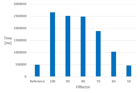
The Reference is the same 1 M dataset, without chemindex, in a table created without fillfactor.

It can be seen that in indexed tables, the speed of the calculation executed in the non-indexed reference table can only be achieved if the fillfactor is set to 50. The 50 % value of the fillfactor means that the memory requirement of the table is approximately doubled compared to the 100 % (or no fillfactor).

Fillfactor 50 is recommended if calculated columns are planned to be added to chemindexed tables.

If no more calculations are planned, the fillfactor can be reset even to 100 by:

ALTER TABLE table_name SET ( fillfactor = 100);
VACUUM FULL table_name;

The possibility of dropping the chemindex before such calculations, and creating them after the calculation is always available.

INSERT INTO TABLE

INSERT INTO table_name (column1,column2,...) VALUES (value1,value2,...);

Example :

INSERT INTO test (id,mol) VALUES (1,'c1ccccc1'); 

MOLECULE INDEX

For indexing a column containing chemical structures the following indextypes are provided:

• chemindex

• sortedchemindex (available from JPC version 2.6)

You can check whether these indextypes exist or not:

SELECT * FROM pg_am WHERE amname='chemindex';
SELECT * FROM pg_am WHERE amname='sortedchemindex';

Indextype chemindex and sortedchemindex can be used in the following way:

CREATE INDEX index_name ON table_name USING chemindex(structure_column_name);
or
CREATE INDEX index_name ON table_name USING sortedchemindex(structure_column_name);

Example:

CREATE INDEX ttest_idx ON ttest USING chemindex(mol);
or
CREATE INDEX ttest_idx ON ttest USING sortedchemindex(mol);

What is the difference between chemindex and sortedchemindex ?

• substructure searching in tables where sortedchemindex is applied gives back the hits quickly in relevance-sorted order, that is hits that are most similar to the query molecule are returned first

• similarity searching in tables where sortedchemindex is applied is also much quicker, especially when narrow similarity threshold is defined

• indexing time is longer (approximately 1.7 times) in case of sortedchemindex

• returning all hits in searches can be faster if chemindex was applied

Do not create indexes of both indextype on the same column simultaneously because it would increase the search time in the given table.

Performance of the indexation process can be increased by setting cache parameters to low memory setup (only substructure fingerprints are cached, molecules and superstructure fingerprints are not cached) and leaving the service JVM heap size at a larger value (option -Xmx). This way garbage collection by the JVM can be optimized and faster indexation can be achieved.

Using the index in any type of searches can be forced by setting enable_seqscan parameter to **OFF ** value in postgres configuration file /etc/postgresql/9.5/main/postgresql.conf .

We suggest closing all transactions and running a VACUUM before creating an index to avoid the calculation of the index data on rows that are being changed in the current transaction. E.g. if a column was added in the current transaction, the index creation time can be almost double of the normal time.

The same logic applies to updating a large number of molecules in an indexed table and then search on the table without closing the transaction and clearing up modification with VACUUM. If possible, update operations and column additions are advised to be performed before adding the chemical index.

Be aware that an ALTERed, not VACUUMed table can contain NULL values in the background and may force the index creation to stop.

See possibilities for finding invalid structures.

How to monitor the CREATE INDEX process

Available from version 5.0.

The view **pg_stat_progress_create_index ** in PostgreSQL database provides information about the status of the CREATE INDEX processes.

The following statement is recommended to run:

SELECT relid, index_relid, command, tuples_total, tuples_done FROM pg_stat_progress_create_index;

In the case of unsuccessful index creation, you can check the How to identify the molecule stopping the create index process? FAQ item

MOLECULE IMPORT

All well known chemical structural data file formats are supported, but we provide functions for importing mol, sdf files.

In case of big files, the postgresql client can run out of memory as the following error message displays:

ERROR:  out of memory
DETAIL:  Cannot enlarge string buffer containing 0 bytes by 1506367917 more bytes

Please, split up the original input file into smaller pieces and import them one after another. (Here is a script tool provided for splitting SD files.)

For importing purposes, usage of scripts consisting of multiple SQL insert statements is not recommended as this operation may be time consuming (especially if the destination table contains a chemical index). To speed up import, it is advisable to use the standard ‘copy’ SQL function or the parse_sdf Chemaxon utility.

From version 20.12, non-valid structures can also be imported and indexed. However, they won't hit any structure, including themselves.

Import from SD file

** Import from local SD/mol files containing added fields besides the chemical structure data **

The content of all the added fields in the SD file will be stored in a hashmap like type column.Optionally selected added fields from the SD file can be stored in separate columns as well.

Follow the next steps:

1. Set the content of the SD file to a variable (e. g.: content )

    \set variable_name `cat sdf_file_name`
   

   Example:

    \set content `cat ~/a.sdf`
   

   You can check the table generated by the parse_sdf function

   SELECT * FROM parse_sdf(:'content');
   

   The parse_sdf function returns the content of the sdf file as a table, which has two columns:

   molSrc = the full sdf source of the original entry in the sdf file

   props = hstore type column, which contains the properties of the sdf entry

   You can also create a table similar to the table created by the parse_sdf function by:

   CREATE TABLE tableName (mol MOLECULE('sample'), p hstore);
   

2. Create a table with create table as:

   CREATE TABLE table_name AS 
       SELECT molSrc::molecule('molecule_type_name') AS structure_column_name[, props ->'sdf_field_name' AS column_name] 
       FROM parse_sdf(:'');
   

   Example:

   CREATE TABLE mysdftable AS 
       SELECT molSrc::molecule('sample') AS mol,
           props -> 'MOLFORMULA' AS formula, CAST(props -> 'CDID' AS INTEGER) AS id
       FROM parse_sdf(:'content');
   

   where

   mysdftable = the name of the table

   mol = the name of the column for storing structural data

   molecule('sample') = the type of column mol

   sample * = molecule type (must be a defined type in /etc/chemaxon/types/ folder *)

   MOLFORMULA = the name of the field in the SD file for storing chemical formula

   formula = the name of the column for storing chemical formula

   CDID = the name of the field in the SD file storing the identifier

   id = the name of the column for storing the identifier integer

   The previous example stored all sdf file content (even the molecule properties) in the mol column. If you do not want to store the whole sdf file content in the mol column just the molecule information (until the M END line), it is also possible in the following way:

Example:

CREATE TABLE mysdftable AS 
    SELECT substring(molSrc,'.*M  END')::molecule('sample') AS mol,
        props -> 'MOLFORMULA' AS formula, CAST(props -> 'CDID' AS INTEGER) AS id
    FROM parse_sdf(:'content');

1. You can also store all properties from the SD file entry in a separate column in the structure table, and later, optionally, add additional columns to separately store selected properties.

   Example:

    \set content `cat ~/a.sdf`
   
   CREATE TABLE mytable AS 
       SELECT molSrc::molecule('sample') AS mol,
           props AS properties 
       FROM parse_sdf(:'content');
   
   ALTER TABLE mytable ADD COLUMN formula TEXT;
   
   UPDATE mytable SET formula = properties -> 'MOLFORMULA'
   

   ​

Collect invalid molecules

Available from version 1.8.

Running the steps below, the molecules in SD/mol files will be checked during the import and the invalid molecules will be stored in a separate table named _error.

Steps:

1. Run the import_sdf.sql script to create function import_sdf . This script file is a customizable tool; you can update it according to your needs.

   \i import_sdf.sql;
   

   {primary}
   Usage of function import_sdf is not recommended in case of tables already containing indexed chemical data as this operation may be time consuming. To speed up import, in this case a temporary table without indexes can be created with import_sdf and then the content of this temporary table can be inserted into the destination table using the following SQL statement:

   insert into <destination table name> select (tt.mol, tt.props, ...) from <temporary table name> tt;
   

   ​

2. Run the following commands including import_sdf function with the appropriate parameters:

    \set <variable_name> `cat <path_to_your_sdf_file>`;
   SELECT import_sdf(:'<variable_name>', '<new_table_name>', '<molecule_type>');
   

   Example:

    \set content `cat ~/a.sdf`;
   SELECT import_sdf(:'content', 'molecules', 'sample');
   

Import from (cx)smiles or (cx)smarts files

• Import from (cx)smiles or (cx)smarts files by the standard copy sql function *

COPY table_name (structure_column_name) FROM 'file_name' (FORMAT csv);

Example:

COPY ttest(mol) FROM '/home/posgresuser/targetfiles/nci-pubchem_1m_unique.smiles' (FORMAT csv);

** Import from (cx)smiles or (cx)smarts files while collecting the invalid molecules **

Available from version 1.8

Running the steps below, the molecules in smiles/cxsmiles/smarts/cxsmarts files will be checked during the import and the invalid molecules will be stored in a separate table named _error **. ** We propose the following two methods: PL/pgSQL script method and SQL commands method.

** ** PL/pgSQL script method ** **

We suggest applying this script method when the server and the client are on the same machine; or at least the molecule files are available on the server and their absolute path is known. Otherwise, apply the steps of SQL commands method.

Steps:

1. Run the import_single_line_format.sql script to create function import_single_line_format. This script file is a customizable tool; you can update it according to your needs.

   \i import_single_line_format.sql;
   

2. Run the following SELECT using import_single_line_format function with the appropriate parameters:

   SELECT import_single_line_format('<absolute_path_to_my_file_on_server>', '<new_table_name>', '<molecule_type>');
   

   Example:

   SELECT import_single_line_format('/home/myuser/molecules.smiles', 'molecules', 'sample');
   

   ​

• SQL commands method *
  1.
  Create a table which will contain the valid molecules

  CREATE TABLE my_table(mol TEXT);
  

1. Import from file

   \COPY my_table FROM '~/molecules.smiles' (FORMAT csv);
   

2. Create and load a table for the invalid molecule sources

   CREATE TABLE my_table_error AS SELECT mol FROM my_table WHERE NOT is_valid_molecule(mol);
   

3. Remove invalid molecules from my_table

   DELETE FROM my_table WHERE mol IN (SELECT mol FROM my_table_error);
   

4. Convert the valid molecule sources into molecule

   ALTER TABLE my_table ALTER COLUMN mol TYPE molecule('sample') USING mol::molecule('sample');
   

Convert molecule source text to molecule from an existing table

Execute the 5^th step of the SQL commands method above.

MOLECULE EXPORT

There is no specific function provided to export your data to a file. However,
it is sometimes required to export your molecule data to a standard format which can be later imported to another tool. This format can be sdf file format which is widely supported.
The following steps describe how to create an sdf file from a column of a table which contains molecule data. The process can be achieved by converting your molecules to a specific file format, copying this data to a file and postprocessing it.

molconvert API is provided to convert between different molecule formats, so you can use molconvert to create an sdffile representation of a structure.

Step by step guide for exporting molecular data to sdf file

Suppose you have a table (mytable) which has some molecule data in the mol column.

1. Create a table (sdfout) which contains molecule data in sdf file format using molconvert API:

create table sdfout as select molconvert(mol, 'sdf') from mytable;

This is a CPU heavy and most probably the slowest step in the export process.

1. Copy the created table to a file with standard sql procedure.

If psql PostgreSQL interactive terminal is available, than that is most probably the best choice, since it supports \copy command which is a frontend (client) copy. (See \copy command in psql client for more information.)
If it is not available the standard SQL server side copy can work as well.

Copy the newly created sdfout table to a file (/tmp/out.sdf):

\copy sdfout to /tmp/out.sdf

The created file contains \n characters instead of newline characters and also extra \n character after the sdf file record separators ($$$$).

1. Convert newline characters and remove superfluous newlines

Use sed command to convert characters and remove superfluous newlines in one step:

sed 's/\\n/\n/g' <out.sdf |sed  '/$$$$/{n;d;}' > out_converted.sdf

The generated out_converted.sdf is a proper sdf file for further usage.

CACHE LOADING

(Available from version 4.3.)

The cache is loaded when the first search is executed, but it can be loaded intentionally at any time using the following statements:

select load_molecule_cache('<index_name>');

select load_fingerprint_cache('index_name>');

Both statements are recommended to be executed if the necessary memory is available.

In the case of low memory setup use only the load_fingerprint_cache function.

MOLECULE FUNCTIONS

Casting a string to any Molecule type defined in /etc/chemaxon/types/

'CCCC'::Molecule('sample')

Postgres type system can cast a string to molecule if it is obvious; if the operation needs a molecule as an input. There are cases when there is no need of explicit casting because of the auto cast mechanism. See details here.

Example:

SELECT 'C' |<| 'CC'::molecule('sample');

Interpreting a string using a specific format

As molecule strings are ambiguous in some cases, it is possible to interpret the given molecule string according to the given molecule format using the molecule(String, String) function:

molecule(structure_string, molecule_format)

where

structure_string = molecule string representation

molecule_format = molecule format string, see file formats

SELECT * FROM table_name WHERE molecule(structure_string, molecule_format) |<| column_name;

A typical usecase is the differentiation between SMILES and SMARTS strings:

• 'CC' with SMILES notation is interpreted as two aromatic or aliphatic carbon atoms connected with a single bond.

• 'CC' with SMARTS notation is interpreted as two aliphatic carbon atoms connected with a single bond.

Example:

SELECT * FROM ttest WHERE molecule('CC', 'smiles') |<| mol;
SELECT * FROM ttest WHERE molecule('CC', 'smarts') |<| mol;

If molecule() function is not applied, the cartridge automatically recognizes the format of the molecule strings and in the case of ambiguous SMILES/SMARTS strings of query structures it handles them as SMILES.

Transformations

Transformation function is provided to transform the molecule structure according to specific needs. Multiple transformation strings can be provided separated by two dots.

query_transform(molecule, 'transformation_string1..transformation_string2')

where

molecule = "molecule string" | Molecule object | table column

transformation string = "dbsmarkedonly" | "ignoretetrahedralstereo" | "ignorecharge" | "ignoreisotope"

Molecule transformation combined with substructure search:

SELECT * FROM ttest WHERE query_transform(molecule, 'transformation string') |<| mol;

• Double bond stereo option: dbsmarkedonly

By default, CIS query matches only with CIS target and TRANS query match es only with TRANS target. If matching of CIS query with both CIS and TRANS targets or matching of TRANS query with both CIS and TRANS targets is aimed, then the query molecule has to be transformed.

The query_transform function with dbsmarkedonly option is provided to accomplish this transformation.

query_transform('query_structure', 'dbsmarkedonly')

Examples:

SELECT * FROM ttest WHERE query_transform('C\C=C\C', 'dbsmarkedonly') |<| mol;
SELECT * FROM ttest WHERE query_transform('C\C=C\C', 'ignoretetrahedralstereo..dbsmarkedonly') |<| mol;

• Ignore tetrahedral stereo search option: ignoretetrahedralstereo (Available from version 5.1.)

Behavior until version 23.17.0: Tetrahedral stereo information stored in the query structure can be ignored during substructure and fullfragment search. The transformation removes the tetrahedral stereo information form the query structures.

Behavior from version 24.1.0: Tetrahedral stereo information stored in the query structure and in the target structures can be ignored during substructure, fullfragment and duplicate search.

query_transform(query_structure, 'ignoretetrahedralstereo')

Examples:

SELECT * FROM ttest WHERE query_transform('C[C@H](n)C(O)=O', 'ignoretetrahedralstereo') |<| mol;

• Ignore charge search option: ignorecharge (Available from version 21.13.)

Behavior until version 23.17.0: Charge information stored in the query structure can be ignored during substructure and fullfragment search. The transformation removes the charge form the query structures.

Behavior from version 24.1.0: Charge information stored in the query structure and in the target structures can be ignored during substructure, fullfragment and duplicate search.

query_transform(query_structure, 'ignorecharge')

Examples:

SELECT * FROM ttest WHERE query_transform('[NH3+]C1=CC=CC=C1', 'ignorecharge') |<| mol;

• Ignore isotope search option: ignoreisotope (Available from version 21.13.)

Behavior until version 23.17.0: Isotope information stored in the query structure can be ignored during substructure and fullfragment search. The transformation removes the isotope form the query structures.

Behavior from version 24.1.0: Isotope information stored in the query structure and in the target structures can be ignored during substructure, fullfragment and duplicate search.

query_transform(query_structure, 'ignoreisotope')

Examples:

SELECT * FROM ttest WHERE query_transform('C1CC[13CH2]CC1', 'ignoreisotope') |<| mol;

Chemical Terms

(Available since version 1.4.)

Calculation of Chemical Terms

Function chemterm makes possible to calculate Chemical Terms.

You may need to purchase separate licenses to apply function chemterm depending on the Chemical Terms used.

chemterm('chemical_term','structure')

where

structure = a molecule string

chemical_term = a Chemical Terms function

The output of function chemterm is one of the following formats:

• string

• molecule string in format mrv

Examples:

SELECT chemterm('name','CCO');
SELECT chemterm('mass()','CCO');
SELECT molconvert(chemterm('canonicalTautomer()','CC(O)=C')::Molecule,'smiles');

Addition of Chemical Terms columns

Chemical Terms columns can be added by using triggers.

See the following code block as an example:

CREATE TABLE test(structure MOLECULE('sample'), molweight NUMERIC);

CREATE OR REPLACE FUNCTION set_molweight()
  RETURNS trigger AS 
$BODY$
BEGIN
     IF NEW.structure is null THEN
      NEW.molweight:=NULL;
    END IF;
    NEW.molweight:=chemterm('mass()',NEW.structure)::real;
    RETURN NEW;
END;
$BODY$
LANGUAGE plpgsql;

DROP TRIGGER IF EXISTS tr_molweight ON test;
CREATE TRIGGER tr_molweight BEFORE INSERT OR UPDATE ON test
 FOR EACH ROW EXECUTE PROCEDURE set_molweight();

UPDATE test SET molweight=chemterm('mass()',structure)::real;

Calculating Chemical Terms on the standardized structure

Chemical Terms is calculated on the input structure without standardization. Combine with the standardize method to calculate Chemical Terms on the standardized structure:

1. Standardize the structure before inserting into the database columns:

   INSERT INTO <your_table> (mol, ... ) VALUES (standardize(<your structure>::Molecule('sample')), ... )
   

2. Store both the not standardized and the standardized structures:

   INSERT INTO <your_table> (mol,standardized_mol ... ) VALUES (<your structure>::Molecule('sample'), standardize(<your structure>::Molecule('sample')), ... )
   

3. Standardize on the fly before calling Chemical Terms:

   select chemterm(<your_chemical_terms>, standardize(<your_structure>::Molecule('sample'))::Molecule);
   

Structure checkers and fixers

The chemterm function makes possible to execute structure checker and fixer operations.

SELECT chemterm('check(''checkerAction’')','molecule');
SELECT chemterm('fix(''checkerAction->fixerAction'')','molecule');

Example:

SELECT chemterm('check(''explicith..doublebondstereoerror'')','[H]C(C)C=C |w:3.2|');
SELECT chemterm('fix(''missingatommap->mapmolecule'')','CCO'); 

See examples in Chemical Terms/Structure checkers documentation page. The available checkers and and their respective fixers are found here.

See how to use custom structure checkers and fixers.

Standardize

(Available since version 4.4.)

Calculating the standardized structure

The standardization steps are determined by the molecule type definition. The returned value is a the standardized structure in MRV format

standardize(molecule)

where

molecule = a Molecule object

Example:

SELECT standardize('C1=CC=CC=C1'::Molecule('sample'));

Molconvert

Conversion to molecule formats

The use of Chemaxon's MolConverter is supported with some limitations:

molconvert('structure', 'format')

where

structure = a Molecule in any of the following formats

format = mrv, mol, rgf, sdf, rdf, csmol, csrgf, cssdf, csrdf, cml, smiles, cxsmiles, abbrevgroup, sybyl, mol2, pdb, xyz, inchi, or name
The export options of the formats can also be applied.

Example:

SELECT molconvert('CC','sdf');
SELECT molconvert('CC','mol:V3');

Conversion to base64 encoded binary formats (image)

Molecules can be converted to binary image formats (png, jpeg, msbmp, pov, svg, emf, tiff, eps) or other binary formats (pdf) in Base64 encoded form.

Example:

SELECT molconvert('CC','base64:png');

Hit highlight

Available from version 21.3.0.

The highlight function compares a query structure with a target structure and highlights the bonds and atoms of the target structure matching with the query structure.

highlight('target_structure','query_structure') 
--- works with default alignment_mode and default color

highlight('target_structure','query_structure','alignment_mode','color')

highlight('target_structure','query_structure','alignment_mode','color','format') 
--- available from version 21.4.0

Examples:

SELECT highlight('CCOCC'::molecule('sample'),'COC');  --- works with alignment_mode OFF and default color blue

SELECT highlight('CCOCC'::molecule('sample'),'COC','rotate','green');

SELECT highlight('CCOCC'::molecule('sample'),'COC','rotate','green','base64:png');
SELECT highlight('CCOCC'::molecule('sample'),'COC','rotate','green','mrv');

Query transformations - dbsmarkedonly and/or ignoretetrahedralstereo - can also be applied:

SELECT highlight('CCOCC', query_transform('COC'::molecule('sample'),'dbsmarkedonly'),'rotate','green');

Three alignment_modes can be applied:

• off [default]

  The hit structure's position is the same as that of the target structure.

• rotate

  The hit structure is rotated till its part corresponding to the query gets the same position as the query structure has.

• partial_clean

  The hit structure's position is partially aligned to the query structure.

The expected color of the highlighted atoms and bonds can also be set.

Available colors: blue [default], black, cyan, dark_gray, gray, green, light_gray, magenta, orange, pink, red, white, yellow

If there is no hit, the output contains the target structure without coloring.

The format can be any format listed above at Molconvert function including the base64 encoded image formats. Default format is MRV.

Molecule validation

Available from version 1.8.

The following function is provided to check the validity of the molecules:

is_valid_molecule(structure_text)

where

structure _text = a Molecule in any of the following formats:

mrv, mol, rgf, sdf, rdf, csmol, csrgf, cssdf, csrdf, cml, smiles, cxsmiles, abbrevgroup, sybyl, mol2, pdb, xyz, inchi, or name

Example:

SELECT is_valid_molecule('CCO');

You can filter out the invalid structures from a table using the following SELECT statement:

SELECT structure_text from mytable where is_valid_molecule(structure_text) = 'f';

Relevance

Function relevance(Molecule) gives back a numeric type value based on the atom counts and further topological features of the molecule. This function can be applied for ordering search results.

Example:

SELECT relevance('CCO'::molecule('sample'));

MOLECULE OPERATORS

The main features of the different search types are available in JChem Query Guide.

The molecule operators work also in tables without chemical index, however, chemical index makes the search operations much faster.

The format of the molecule strings are automatically recognized. The ambiguous molecule strings - for example 'CCC' - which can be either SMILES or SMARTS are interpreted in the query structures as SMILES.

JDBC Caution

Please take into account the JDBC related recommendation when implement structure searches.

Substructure search

Substructure search is performed using the symmetrical sub-/super-structure search operator: |<|.

SELECT * FROM table_name WHERE query_structure |<| structure_column_name;
SELECT * FROM table_name WHERE structure_column_name |>| query_structure;

SELECT * FROM table_name WHERE query_mol |<| target_mol;
SELECT * FROM table_name WHERE target_mol |>| query_mol;

where

query_mol = "molecule string" | Molecule object | table column

target_mol = "molecule string" | Molecule object | table column

Query features and Markush features are not supported on target_mol.

Examples:

SELECT '[#6]-[#6]' |<| 'CC'::Molecule('sample');

SELECT * FROM ttest WHERE 'c1ccccc1' |<| mol;

SELECT * FROM ttest WHERE 'testmol
Mrv0541 01211514572D          

  3  2  0  0  0  0            999 V2000
    1.2375   -0.7145    0.0000 C   0  0  0  0  0  0  0  0  0  0  0  0
    1.9520   -1.1270    0.0000 C   0  0  0  0  0  0  0  0  0  0  0  0
    2.6664   -0.7145    0.0000 C   0  0  0  0  0  0  0  0  0  0  0  0
  1  2  1  0  0  0  0
  2  3  1  0  0  0  0
M  END
' |<| mol;

See also molecule functions about defining the query structure format.

In order to get the hits quickly and sorted by relevance, please, create index on the structure column using sortedchemidex indextype instead of chemindex indextype.

See section Relevance sorting for more information.

Use of prepared statements

In case you plan to apply prepared statements for substructure search, please, take into account the comments relating PostgreSQL Server Prepared Statements like "Server side prepared statements are planned only once by the server. This avoids the cost of replanning the query every time, but also means that the planner cannot take advantage of the particular parameter values used in a particular execution of the query. You should be cautious about enabling the use of server side prepared statements globally. "

Superstructure search

Superstructure search is performed using the sub-/super-structure search operator: |>|.

SELECT * FROM table_name WHERE query_structure |>| structure_column_name;
SELECT * FROM table_name WHERE structure_column_name |<| query_structure;

SELECT * FROM table_name WHERE query_mol |>| target_mol;
SELECT * FROM table_name WHERE target_mol |<| query_mol;

where

query_mol = "molecule string" | Molecule object | table column

Query features and Markush features are not supported on query_mol.

target_mol = "molecule string" | Molecule object | table column

Example:

SELECT * FROM ttest WHERE 'CCC' |>| mol;

Full fragment (exact fragment) search

From version 20.15 the following syntax is available for full fragment search.

SELECT * FROM table_name WHERE query_structure |<=| structure_column_name;
SELECT * FROM table_name WHERE structure_column_name |=>| query_structure;

Example

SELECT * FROM ttest WHERE 'CCC' |<=| mol;
SELECT * FROM ttest WHERE mol |=>| 'CCC';

For versions older than 20.15.0, see the syntax in Deprecated API documentation page.

Duplicate search

Duplicate search is performed using the |=| operator.

SELECT * FROM table_name WHERE query_structure |=| structure_column_name;
SELECT * FROM table_name WHERE structure_column_name |=| query_structure;

Example:

SELECT * FROM ttest WHERE 'CCC' |=| mol;

Tautomer search

If you want to execute tautomer search in column storing the molecules, the molecule type of the column must have one of the following **tautomer = ** tautomer mode.

tautomer = GENERIC tautomer mode

How generic tautomer search executes the query and target matching?

• in duplicate and full fragment search the generic tautomer - representing all theoretically possible tautomers - of the query and the generic tautomer of the target is compared
• in substructure search the query itself is matched with the generic tautomer of the target
• in superstructure search the target itself is matched with the generic tautomer of the query

*tautomer = CANONIC_GENERIC_HYBRID ** tautomer mode (deprecated in version 23.12)

*tautomer = NORMAL_CANONIC_GENERIC_HYBRID ** tautomer mode (available from version 23.12)

It is a hybrid tautomer search mode. The query structure is compared to the generic tautomer of target at substructure search, while normal canonical tautomers are compared at duplicate search. In full fragment search from version 20.12 to 20.14 the generic tautomer of the target is used, while from version 20.15 normal canonical tautomers are compared.

**tautomer = NORMAL_CANONIC_NORMAL_GENERIC_HYBRID ** tautomer mode (available from version 23.12)

It is a hybrid tautomer search mode. The query structure is compared to the normal generic tautomer of target at substructure search, while normal canonical tautomers are compared at duplicate and full fragment search.
The normal generic tautomer represents a chemically more feasible set of tautomers than the generic tautomer which represents the combinatorically possible tautomers.


See details and differences between tautomers here.

Limitations:

• SMARTS atoms and SMARTS bonds in the query structures are not supported.

• The use of bond lists in query structures may slow down the search.

• From version 22.22.0 the normal canonical tautomer form only for structures having max 100 heavyatoms is taken into account in tautomer search, by default. The limit value is configurable

Similarity search

There are some differences between the similarity scores of the new method and of the old methods of JPC. The new method works on the standardized chemical structures while the old methods do not use the standardized format, only the original chemical structures. The new method provides better performance than the old methods. None of them supports query features on the query molecules, but they handle their presence differently.

New method

Available from JPC version 2.5. This new method provides better performance than the old methods, and there is no need to add extra fingerprint column to the table.

You can select those molecules and their similarity value from a table whose similarity value relating the given query structure is greater (or smaller) than a given similarity threshold value.

For this purpose the sim_filter or the sim_order type can be applied as shown below in the examples. The use of the sim_filter * type results unsorted output, while the use of the *sim_order type results sorted output.

For retrieving the most (or less) similar target molecules ** sorted by their similarity values, the *sim_order type must be applied and the *LIMIT n condition can also be useful for better performance if only the most similar (or dissimilar) molecules are required.

SELECT field1, field2, structure_column_name |~| 'query_structure' FROM table_name 
    WHERE ('query_structure', similarity_value)::sim_filter operator structure_column_name;

SELECT field1, field2, structure_column_name |~| 'query_structure' FROM table_name 
    WHERE ('query_structure', similarity_value)::sim_order operator structure_column_name LIMIT n;

where

similarity_value is the dissimilarity threshold, a number between 0 and 1

operator can be ** |<~|** (meaning similarity value is greater than or equal) or |~>| (meaning similarity value less than or equal)

Examples :

SELECT mol FROM moltable WHERE ('CCC', 0.8)::sim_filter |<~| mol;
SELECT mol, mol |~| 'CCC' FROM moltable WHERE ('CCC', 0.8)::sim_filter |<~| mol;
SELECT count(*) FROM moltable WHERE ('CCC', 0.8)::sim_filter |<~| mol;

SELECT mol, mol |~| 'CCC' FROM moltable WHERE ('CCC', 0.8)::sim_order |<~| mol LIMIT 20;
SELECT mol, mol |~| 'CCC' FROM moltable WHERE ('CCC', 0.2)::sim_order |~>| mol LIMIT 20;

Limitations:

• Query structures with query features (like list atoms, query atoms, query bonds, ... ) are not supported.
  

Old methods

The old methods are removed.

Reaction search

Available from version 2.3.

The following search types are supported not only for molecules but for reactions as well.

• substructure search

• superstructure search

• full fragment search

• duplicate search

Reaction specific query features - like different positions of the reaction arrow - are taken into account. See examples here in Table 2.

NOT (substructure, duplicate, etc.) search conditions

There are no specific operators for NOT (substructure, duplicate, etc.) search conditions. The SQL language offers some techniques to implement it, and be careful, because in many cases the performance impact can be huge.

1. using NOT keyword: simple to write and maintain, but it doesn't use the index, so it usually doesn't perform well, and only advised if there are some other, very selective conditions in the query:

SELECT * FROM table_name WHERE NOT (query_structure |<| structure_column_name);

1. using EXCEPT keyword: more difficult to write and maintain, but it uses the index, so it usually performs well, and is advised unless there are other, very selective conditions in the query:

SELECT * FROM table_name
EXCEPT
SELECT * FROM table_name WHERE query_structure |<| structure_column_name;

Connection handling during searching

After retrieving the desired hits, the SQL connection needs to be closed in order to close the search on the jchem-psql server side. You can achieve this by having autocommit switch on or by calling commit explicitly.

Combination of structure query AND structure/non-structure query

• WHERE condition referring to more than one column containing chemical structure data is not supported.

• WHERE condition referring to one structure column and one or more columns containing non-chemical structure data is supported.
  

Relevance sorting

Relevance sorting of substructure search results is provided by JPC. The new method sorts the hit molecules according to the similarity between them and the query structure. This new method is much faster than the old method which sorts by relevance function. There can be some difference between the order of the hit molecules retrieved by the two methods.

Relevance sorting by using order by molecule column

This simple method is introduced in version 2.6.

In order to get the results quickly and sorted by relevance, the column storing the chemical structures must be indexed with sortedchemindex.

For executing substructure search the use of ORDER BY is essential and the LIMIT n parameter is recommended.

Example (assuming table "test" has column "mol" of type Molecule):

CREATE INDEX test_idx on test using sortedchemindex(mol);

SELECT mol FROM test WHERE 'c1ccccc1' |<| mol ORDER BY mol LIMIT 100;

ORDER BY is only available for substructure search. In case of other search types, error message is given.

Applying ORDER BY in searches containing joins of several constraints, the execution plan optimizer of PostgreSQL may decide to choose a plan where a final sorting step is involved instead of keeping the original sorting order available in sortedchemindex. This may take very long time because sorting requires very expensive comparisons. In this case we advise to force the planner to choose a plan without sort by executing the command

SET enable_sort=OFF;

It is necessary because PostgreSQL does not take into account the comparator function's cost in the cost of sorting.

Relevance sorting by using relevance function

Relevance sorting by using relevance function is deprecated.

AUXILIARY FUNCTIONS

Debugging

Raising the log level of the psql-client for debugging purposes:

SET client_min_messages to debug;

Performance log

You can log the performance of the current session as:

SELECT * FROM perf_out();

You can clear the log as (available since version 1.4):

SELECT perf_reset();

See the description of the parameters listed in the output of perf_out().

Performance tuning of combined queries

Available since version 1.4.

The performance of searching with combined queries - when chemical structure query condition is combined with a non-structure query condition - might be improved by executing the following calibration steps.

1. Prerequisite: the column structure_column_name in table table_name used for the calibration must be indexed using indextype chemindex or ** sortedchemindex.**

2. Calibration of cost factors

   select calibrate_cost_factors('table_name', 'structure_column_name', 'query_structure');
   

   where

   query_structure is an optional parameter. If not specified, chlorobenzene (Clc1ccccc1) is used by default.

   {info}
   The applied query_structure is an important key factor of the calibration. The best specified query_structure has almost the same (± 10%) estimated selectivity in the given table as the number of its search hits. We recommend the next explain statement to run in order to get the estimated selectivity. The number of rows given in the output of the next statement is the estimated selectivity.

   explain select * from table_name where 'query_structure' |<| structure_column_name;
   

   ​

   {primary}
   In order to get better performance, you may need to increase the default_statistics_targetvalue for PostgreSQL analyzer. Its default value 100 can be increased to maximum 10000.
   

3. Application of the calibrated cost factors

   Please follow the suggested solutions given in the output of the select calibrate_cost_factors statement.

   Example up to version 2.6:
   To set the values permanently, add the lines

   chemaxon.cost_slope_factor = -5.14e-07
   
   chemaxon.cost_intercept_factor = 0.03866
   

   to the PostgreSQL configuration file (e.g.: /etc/postgresql/9.5/main/postgresql.conf).

   To set values only for the current session, execute the following commands:

   SET chemaxon.cost_slope_factor = -5.14e-07;
   
   SET chemaxon.cost_intercept_factor = 0.03866;
   

   Example from version 2.7:

   To set the values permanently, add the lines

   chemaxon.index_screen_factor = 0.00002
   
   chemaxon.index_abas_factor = 0.00895
   
   chemaxon.seq_screen_factor = 0.00076
   
   chemaxon.seq_abas_factor = 0.26312
   

   to the PostgreSQL configuration file (e.g.: /etc/postgresql/9.5/main/postgresql.conf).

   To set values only for the current session, execute the following commands:

   SET chemaxon.index_screen_factor = 0.00002
   
   SET chemaxon.index_abas_factor = 0.00895
   
   SET chemaxon.seq_screen_factor = 0.00076
   
   SET chemaxon.seq_abas_factor = 0.26312
   

   ​