Atom-by-Atom Search

Traditionally substructure search is executed by performing a labeled graph
matching algorithm. There are multiple algorithms for matching labeled graphs,
but the method developed by Ullmann [^1] is the one which has been widely used
in the case of chemical substructure matching in the last 20 years. In 2004
the so-called VF2 algorithm [^2] was published with the advantage of higher
performance in the case of typical chemical graphs.

Ullmann's algorithm

Ullmann's algorithm builds a mapping matrix (M) that defines possible query-
target atom mapping pairs. The algorithm iterates on this matrix and clears
infeasible query-target atom mappings based on local properties (atom number,
number of connections, etc.) and neighbor connectivity as long as the matrix
is changed. After the iteration is finished (the matrix is not changing any
more), a backtracking algorithm is performed to find a specific query-target
atom mapping. A feasible mapping is selected, then the matrix is copied and
iteratively cleared again based on local properties and neighbor
connectivities. If the clearing process leads to a zero row - no possible
matches for a query atom - we step back to the previous query atom and search
for another feasible target match if any. This selection and matrix clearing
is iterated recursively until all atoms are matched or there is no possible
match for the specific query target pair.

This algorithm is working well for chemical graphs, although it may explode
exponentially on general graphs. In optimal case, its computational cost is
going with the order of the square of query atom count multiplied by target
atom count. The memory allocation is in the order of the mapping matrix (M)
multiplied by the number of query atoms: square of query atom count multiplied
by target atom count. For large (peptide-like) structures, this large memory
requirement should be considered.

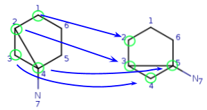
Simple example for graph isomorphism (duplicate match)

The following example describes the matrix clearing phase of Ullmann's
algorithm. In this case, the matrix clearing phase results in a well-defined
mapping, so no further recursion is needed.

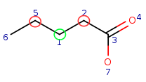
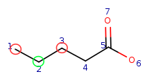
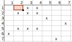
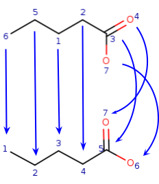
Query:

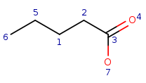
Target:

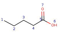
Local atom properties:

Local atom property	Atom property image	Query atom indexes having the given atom property	Target atom indexes having the given atom property
Carbon atom with one single bond connection		q6	t1
Carbon atom with two single bond connections		q5, q1, q2	t2, t3, t4
Carbon atom with three connections including one double bond and two single bonds		q3	t5
Oxygen atom with one single bond connection		q7	t6
Oxygen atom with one double bond connection		q4	t7

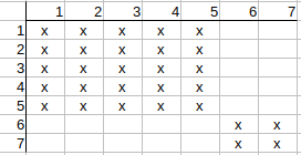
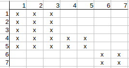
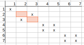
Initial mapping matrix with local property matching:

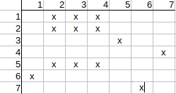
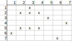
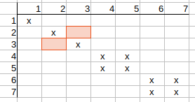
Checking possible q1-t2 mapping.

The neighbors of q1 are q2, q5.

The neighbors of t2 are t1, t3.

Checking q2 (row) in the matrix, we can see that it has a t3 match, but no t1
match.

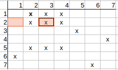
This means that the other neighbor of q1, i.e. q5, should have a t1 match, but
it has not either.

That is, the neighbors of q1 cannot be mapped to the neighbors of t2, so the
possible q1 match to t2 can be deleted.

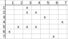
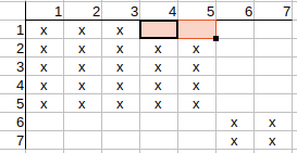
Next we check q1-t3 mapping. The neighbors of q1 are q2, q5. The neighbors of
t3 are t2, t4.

q2 has t2, t4 matches and q5 has t2, t4 matches. All neighbors are matched,
nothing to be cleared.

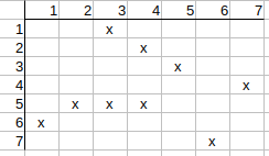
Next we check q1-t4 mapping. The neighbors of q1 are q2, q5. The neighbors of
t4 are t3, t5.

q2 has a t3 match, but no t5 match, so q5 should have a t5 match, which it has
not. We could not identify the proper matches for q1 neighbors to t4
neighbors, so this possible mapping can be deleted.

Similarly, we check q2 possible mapping to t2. The neighbors of q2 are q1, q3,
and the neighbors of t2 are t1, t3.

q1 has t3 match, but no t1 match, so q3 needs to have t1 match, which it has
not, so q2 possible match to t2 can be deleted.

Checking q2 possible match to t3. The neighbors of q2 are q1, q3, and the
neighbors of t3 are t2, t4. q1 has neither t2 nor t4 match, so q2 possible
match to t3 can be deleted.

Checking q2 possible match to t4. The neighbors of q2 are q1, q3, and the
neighbors of t4 are t3, t5. q1 has t3 match and q3 has t5 match. All neighbors
are matched, nothing to be cleared.

Similarly, checking q3 possible match to t5 and q4 possible match to t7, we
notice that all neighbors are matched and nothing to be cleared.

Checking q5 possible match to t2. The neighbors of q5 are q1, q6, and the
neighbors of t2 are t1, t3. q1 has t3 match and q6 has t1 match.

Checking q5 possible match to t3. q5 neighbor q1 does not match any of t3
neighbors (which are t2, t4), so q5 possible match to t3 can be deleted.

Similarly, checking q5 possible match to t4, we observe that q5 possible match
to t4 can also be deleted.

One can continue with q6 and q7 similarly and can observe that no further
possible matches will be deleted.

Now we have to repeat the clearing process to check the remaining mappings of
all query atoms. This is necessary as later clearings may have disabled the
matching of previous rows (e.g. clearing q5-t3 match may disable q2-t4 match).
The clearing (originally called refinement) process is repeated till there is
a full map checking that keeps the map unchanged. In the presented example,
the map is unchanged in the second iteration.

Since all matrix rows and columns have a single possible match, we have the
exact matching information, which provides query-target atom mapping+.

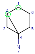
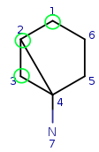
Another example where selection from different possibilities and recursion is
needed:

Query: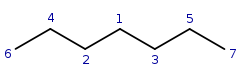
Target:

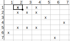
Initial matrix with local property matching:

Checking q1-t1 possible match. q1 neighbors are q2, q3, and t1 neighbors are
t2, t3.

q2 has t2 match and q3 has t3 match, so there is nothing to update on the
matrix.

Checking q1-t2 possible match. q1 neighbors are q2, q3, and t2 neighbors are
t1, t4.

q2 has t1 match and q3 has t4 match, so there is nothing to update on the
matrix.

Checking q1-t3 possible match. q1 neighbors are q2, q3, and t3 neighbors are
t1, t5.

q2 has t1 match and q3 has t5 match, sothere is nothing to update on the
matrix.

Checking q1-t4 possible match. q1 neighbors are q2, q3, and t4 neighbors are
t2, t6.

q2 has t2 match, but q3 has no t6 match. q2 has no t6 match either. So q1-t4
possible match can be deleted.

Checking q1-t5 possible match. q1 neighbors are q2, q3, and t5 neighbors are
t3, t7.

q2 has a t3 match, but q3 has no t7 match. q2 has no t7 match either. So q1-t5
possible match can be deleted.

Continuing with q2, q3, we see that their possible matches to t4 and t5 can
also be deleted.

Continuing with q4, q5, we see that thier possible matches to t1, t2, t3 can
also be deleted.

Checking q6 and q7, we observe that no possible match can be deleted.

Since there were changes in the matrix, we need to check it again to see if
other possible matches can be cleared.

Checking q1-t1 possible match again. q1 neighbors are q2, q3, and t1 neighbors
are t2, t3.

q2 has t2 match and q3 has t3 match, so there is nothing to update on the
matrix.

Checking q1-t2 possible match. q1 neighbors are q2, q3, and t2 neighbors are
t1, t4.

q2 has t1 match but q3 has no t4 match, so t2 possible match can be deleted.

Checking q1-t3 possible match. q1 neighbors are q2, q3, and t3 neighbors are
t1, t5.

q2 has t1 match but q3 has no t5 match, so t3 possible match can be deleted.

Continuing with q2, q3, we see that their possible matches to t1 can also be
deleted.

Checking q4, q5, q6, q7, we see that no further possible matches can be
deleted.

Since we have modified the matrix in this iteration as well, we check it again
from the beginning and realize that no further possible matches can be
deleted.

Now, we can see that we have rows where multiple possible matches are
available. Here comes the backtracking phase where we have to select from the
possible matches and perform the matrix clearing again.

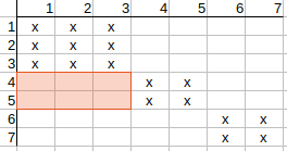
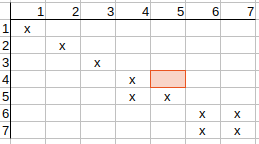
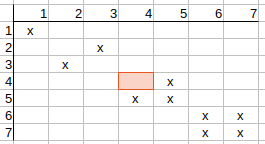
Selecting the possible q2-t2 match and deleting the directly conflicting
possibilities (q2-t3, q3-t2), we get the following matrix:

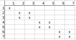
Iterating on the matrix and checking possible matches, we see that q1-t1,
q2-t2, q3-t3 possible matches remain.

q4-t4 possible match also remains, since q4 has neighbors q2, q6, and t4 has
neighbors t2, t6, and q2 has t2 match, q6 has t6 match, so there is nothing to
update on the matrix.

Checking q4-t5 possible match. q4 neighbors are q2, q6, and t5 neighbors are
t3, t7.

q2 has neither t3 nor t7 matches, so t5 possible match can be deleted.

Similarly q5-t4, q6-t7, q7-t6 possible matches can also be deleted.

Iterating on the matrix again (since it has been changed) and rechecking
possible matches, we see that the matrix does not change anymore, so we found
a feasible solution.

It is worth mentioning that when we entered the backtracking phase, we had an
option to choose q2-t3 instead of q2-t2. Let's see what happens if we select
this option.

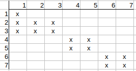
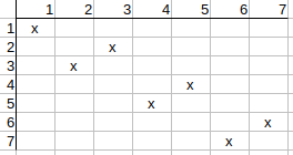
In this case, we delete q2-t2 and q3-t3 and clear the matrix:

q1-t2, q2-t3, q3-t2 possible matches remain.

Checking q4-t4 possible match. q4 neighbors are q2, q6, and t4 neighbors are
t2, t6. q2 has neither t2 nor t6 match, so t4 possible match can be deleted.

Similarly, q4-t5 possible match remains, q5-t5 and q6-t6 possible match can be
deleted, q6-t7 and q7-t6 possible matches remain, and q7-t7 possible match can
be deleted.

Iterating on the matrix again (since possible matches were removed) and
rechecking possible matches, we realize that the matrix does not change
anymore, so we found another feasible solution.

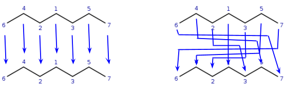
Using different possible matching options when entering into the recursion
phase, we found two different mappings of query atoms to target atoms:

VF2 algorithm

The VF2 algorithm does not build any matrix, its initialization cost is much
smaller compared to Ullmann's algorithm.

It starts with an atom (q1) and matches it (based on local properties) to a
target atom (t1). Takes another connected query atom (q2) and matches it to
another target atom (t2), then checks if all neighbors of q2 that are
previously mapped to target atoms are also connecting to t2all previously
mapped neighbors of q2 are mapped to neighbors of t2.

Let's see a simple example:

Query:

Target:

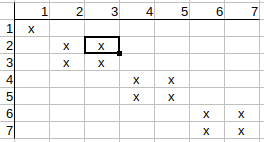
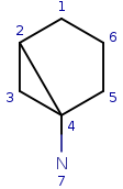
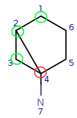
Start with query atom index 1 (q1) that matches (based on local atom
properties) to target atom index 1 (t1). Take a neighbor of q1, query atom
index 2, and try to match it to target atom index 2 (t2). Since q2 has three
connections and t2 has just two, it is not a valid match, similarly q2 cannot
be matched on t6.

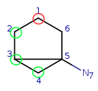
Query:

Target:

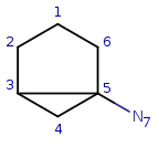
Step back to the beginning and try matching q1 to t2. All local properties are
matching, so continue with q1 neighbor q2. Try q2 with the first available
target: t1. They fail to match due to the difference in the number of
connections. Try q2-t3 match, which is correct. Check if q2 has mapped
neighbors. Yes, it has the q1 which is mapped to t2, that is the neighbor of
t3.

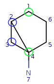
Query:

Target:

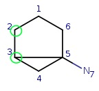
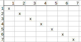
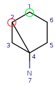
Everthing is fine so far, so step forward. Take q2 neighbor q3 and try to
match it to t1. They are matching locally, so check their neighbors. q3 has
mapped neighbor q2. q2 mapped to t3, but that is not a neighbor of t1, so the
matching failed.

Try to match q3 to t4. All local properties are matching, so it is a possible
match, and the neighbors are also matching. q3 mapped neighbor is q2, q2 map
is t3, and t3 is a neighbor of t4.

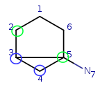
Query:

Target:

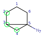
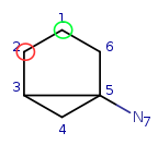
Let's go further to q4. Try to map it to t1. This attempt fails locally due to
the number of connections.

Query:

Target:

Try to map q4 to t5. It is a possible match locally, so check the neighbors.
q4 has mapped neighbors: q3 and q2. The corresponding maps are q3-t4, q2-t3.
And both t3 and t4 are neighbors of t5, so the matching is accepted.

Query:

Target:

We have four matching atom pairs so far: query atoms 1, 2, 3, 4 are mapped to
target atoms 2, 3, 4, 5.

The algorithm continues similarly until all query atoms are mapped.

The VF2 algorithm was developed further in 2015 to VF2 Plus [^3] and VF2 Plus
was developed even further in 2018 to VF2++ [^4].

Using the importance of the node order and using more efficient cutting rules,
the VF2++ algorithm is able to match graphs of thousands of nodes in
practically near-linear time including preprocessing. It is shown that VF2++
consistently outperforms VF2 Plus on biological graphs. In case of random
sparse graphs, VF2++ is faster than VF2 Plus, and it also has a practically
linear behavior both in the case of induced subgraph and graph isomorphism
problems.

Atom-by-atom search in large target sets

In practice, when there are many target molecules to be checked, these graph
matching algorithms are not used alone. The target molecule set is prefiltered
for possible matches, and the remaining candidates are provided for the
specific graph matching algorithm. This filtering is typically executed using
substructure preserving fingerprints. For both the query and the target
structures, the substructure preserving fingerprints are calculated, and if
all bits that are set in the query fingerprint are also set in the target
fingerprint, then it identifies a hit candidate. So in a typical scenario, the
substructure search is executed in two phases. First, the so-called screening
phase is executed, where the hit candidates are identified, which is followed
by the atom-by-atom matching (graph matching) phase. The screening phase is
orders of magnitude faster than the atom-by-atom search phase, as it only
performs fingerprint comparison. The target fingerprints can be calculated
upfront and can be stored in memory for optimal performance. If the
selectivity of the fingerprint is not high enough, additional properties can
be taken into consideration to reduce the number of hit candidates. However,
even in case of good selectivity, one might not want to execute all atom-by-
atom matchings, since the desired result count - e.g. which can be digested by
a human - is much smaller compared to the actual hit count. As a simple
example, we can imagine searching with a very common substructure (like a
benzene ring) in a target set containing 1M structures. In a typical molecule
set, at least 50% of the structures contain benzene ring. Would a chemist need
to have all the ~500k hits? Not always, in the case of a user facing
application, only the first 10-50 hits are presented, but these hits should be
the most valuable ones. In this case, the ordering of the possible hits by
similarity to the query structure can help to avoid superfluous (and long
running) atom-by-atom searches.

Implementation at Chemaxon

In Chemaxon's solution, custom implementations are applied to improve
fingerprint selectivity which is needed indeed to be able to support wide
range of query
features.
In our new search solutions, the ordering of the hits is based on the query-
target similarity value, and either Ulmann's algorithm or an internally
improved VF2++ graph matching algorithmis used depending on the complexity of
the query structure to achieve the fastest atom-by-atom matching speed.

References:

[^1]: J. R. Ullmann, An algorithm for subgraph isomorphism, Journal of the ACM (JACM), Volume 23 Issue 1, Pages 31-42, 1976.

[^2]: L. P. Cordella, P. Foggia, C. Sansone, M. Vento, A (sub)graph isomorphism algorithm for matching large graphs, IEEE Transactions on Pattern Analysis and Machine Intelligence Volume 26 Issue 10, Page 1367-1372, 2004.

[^3]: V. Carletti, P. Foggia, M. Vento, VF2 Plus: An improved version of VF2 for biological graphs, Conference: Graph-Based Representations in Pattern Recognition, At Beijing, 2015.

[^4]: Alpar Juttner, Peter Madarasi, VF2++ An improved subgraph isomorphism algorithm, Discrete Applied Mathematics, Volume 242, Pages 69-81, 2018.